Track 2: Marine cargo vessel power estimation¶

Task¶

Power Estimation is a scalar regression task which involves predicting the current power consumption of a merchant vessel at a particular timestep based on tabular features describing vessel and weather conditions. A probabilistic regression model would yield a probability density over the power consumption. The prediction of the output is mostly attributed to the current timestep, but due to transient effects (e.g inertia) and hull fouling previous timesteps can also affect target power.

Data¶

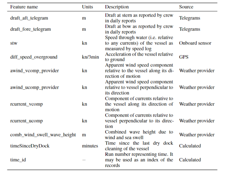
The Shifts vessel power estimation dataset consists of measurements sampled every minute from sensors on-board a merchant ship over a span of 4 years, cleaned and complemented with weather data from a third-party provider. The task is to predict the ships main engine shaft power, which can be used to predict fuel consumption given an engine model, from the vessel's speed, draft, time since last dry dock cleaning and various weather and sea conditions. The following table summarizes the features available in the time-series given in a tabular form.

Uncertainty in the data arises due to sensor noise, measurement and transmission errors, and uncertainty in historical weather.  Distributional shift arises from hull performance degradation over time due to fouling, sensor calibration drift, and variations in non-measured sea conditions such as water temperature, salinity etc. which vary in different regions and times of year.

To provide a standardized benchmark, we have created a canonical partition on the dataset into in-domain train, development and evaluation as well as distributionally shifted development and evaluation splits, as is the standard in Shifts. The dataset is partitioned along two dimensions: wind speed and time, as illustrated in the following figure. Wind speed serves as a proxy for unmeasured components of the sea state, while partitioning in time aims to capture effects such as hull fouling and sensor drift.

In addition to the standard canonical benchmark we are providing a synthetic benchmark dataset created using an analytical physics-based vessel model. The synthetic dataset contains the same splits and input features as in the canonical dataset, but the target power labels are replaced with predictions of a physics model. Given that vessel physics are fairly well understood, it is possible to create a model of reality which captures most relevant factors of variation and model them robustly.

A significant advantage of the synthetic dataset is that is allows generating a generalisation dataset that can cover the  *convex hull *of possible feature combinations. Specifically, additional data points (2.5 million) are created by applying the model to input features independently and uniformly sampled from a predefined range. The idea is to sample from the convex hull of the full range of possible conditions, so all samples are i.i.d., and rare combinations of conditions are equally represented. For example, vessels are less likely to adopt high speeds in severe weather, which could lead ML models to learn a spurious correlation. This bias would not be detected during the evaluation on real data as the same correlation would be present. Evaluating a candidate model on this generalisation task thus tests its ability to properly disentangle causal factors and generalise to unseen conditions. This generalisation set can enable assessing model robustness with greater coverage, even if on a simplified version of reality.

The real and synthetic datasets can be used together. The real-world performance and hyper-parameter exploration can be done using the real data, while the synthetic generalisation set can be used to more broadly assess generalisation to unseen feature variations.

Evaluation¶

Predictive performance is assessed using the standard metrics: Root Mean Square Error (RMSE), Mean Absolute Error (MAE) and Mean Absolute Percentage Error (MAPE). Area under Mean Square error (MSE) and F1 retention curves [Malinin, 2019, Malinin et al., 2021] is used to assess jointly the robustness to distributional shift and uncertainty quality. The respective performance metrics are named R-AUC and F1-AUC. Following the methodology proposed by Malinin et al., 2021, we use the MSE as the error metric and for F1 scores we consider acceptable predictions those with MSE<(500kW)^2. As the uncertainty measure, we use the total variance (i.e. the sum of data and knowledge uncertainty [Malinin, 2019]). A good model should have a small R-AUC and large F1-AUC. 

Baseline¶

We provide a deep ensemble of 10 Monte-Carlo dropout neural networks as a baseline.  The ensemble method yields both improvement in robustness and interpretable estimates of uncertainty. Each ensemble member predicts the parameters mean and standard deviation of the conditional normal distribution over the target (power) given the input features. As a measure of uncertainty we use the total uncertainty, that is the sum of the variance of the predicted mean and the mean of predicted variance across the ensemble. 

The deep ensemble members have the same architecture: 2 hidden layers with 50 and 20 nodes and softplus activation function. The output layer has 2 nodes and a linear activation function. To satisfy the constraint of positive standard deviation the second output is fed through a softplus function and a constant 10^(-6) is added for numerical stability as proposed by Lakshminarayanan et al., 2017. During inference we sample 10 times each member of the ensemble (100 samples in total) to estimate the epistemic uncertainty.  For optimization, we use the negative log likelihood loss function and the Adam optimizer with a learning rate of 10^(-4). The number of epochs is defined by early stopping, monitoring the mean absolute error (MAE) of the dev_in set. The models are implemented in PyTorch.

Get started¶

We provide a full set of code and tutorials at GitHub that step you though the process required to develop and evaluate your models locally. Via the tutorials you are able to reproduce the baseline deep ensemble we provide and evaluate its performance.

Ready to submit? Visit the submission page explaining how to build and submit you docker model.

References¶

1. [Malinin et al., 2021] Andrey Malinin, Neil Band, Yarin Gal, Mark Gales, Alexander Ganshin, German Chesnokov, Alexey Noskov, Andrey Ploskonosov, Liudmila Prokhorenkova, Ivan Provilkov, Vatsal Raina, Vyas Raina, Denis Roginskiy, Mariya Shmatova, Panagiotis Tigas, and Boris Yangel, “Shifts: A dataset of real distributional shift across multiple large-scale tasks,” in Thirty-fifth Conference on Neural Information Processing Systems Datasets and Benchmarks Track (Round 2), 2021.
2. [Malinin, 2019] Andrey Malinin, Uncertainty Estimation in Deep Learning with application to Spoken Language Assessment, Ph.D. thesis, University of Cambridge, 2019.
3. [Lakshminarayanan et al., 2017] B. Lakshminarayanan, A. Pritzel, and C. Blundell, “Simple and Scalable Predictive Uncertainty Estimation using Deep Ensembles,” in Proc. Conference on Neural Information Processing Systems (NIPS), 2017.